
Procedures: Experiment A: XRF as a technique for monitoring changes in the elemental content of paper during washing
- Tim Barrett, director, UICB Paper Facilities, University of Iowa Center for the Book
- Irene Brückle, professor of conservation, State Academy of Fine Arts, Stuttgart, Germany
- Yvonne Hilbert, graduate student in conservation, State Academy of Fine Arts Stuttgart, Germany
- Robert Shannon, applications physicist, Bruker Elemental
- Aaron Shugar, assistant professor, Art Conservation Department, Buffalo State College
- Jennifer Wade, program director, Deep Earth Section of the Division of Earth Sciences, Division of Geosciences, National Science Foundation; formerly: research chemist, Preservation Research and Testing Division, Library of Congress
- Josefine Werthmann, graduate student in conservation, State Academy of Fine Arts Stuttgart, Germany
Abstract
The goals of this project were to monitor changes in calcium (Ca), magnesium (Mg), aluminum (Al), potassium (K), sulfur (S), copper (Cu), iron (Fe), and zinc (Zn) concentration in paper before and after standardized washing procedures, and then to determine if XRF analysis can accurately monitor those changes nondestructively. Six historical specimens and three controls were used in the experiment. All were exposed to seven aqueous treatments. Each specimen was analyzed before and after treatment, using a Bruker Tracer III-V handheld XRF instrument fitted with a special accessory. Sample material was then cut from each specimen in the exact location of the XRF analyses, and ICP-OES destructive methods were used to determine the concentrations in ppm of the elements of interest. During the experiment, 992 XRF and 81 ICP-OES analyses were executed. If we assume the Ca in the historical specimens is tied to desirable alkalinizing compounds and Al is tied to residual alum in the paper, the ICP-OES data suggest aqueous treatment may be removing more and replacing less Ca than desired and also removing less Al than desired. These trends deserve additional research attention. The XRF spectra and the ICP-OES data were used to create a calibration. For Ca, K, and S, we believe the calibration allows us to estimate ppm concentrations with a precision of +/-20% at a 90% confidence level when concentrations are near 1,000 mg/kg (ppm). For Fe, our precision is closer to +/-18% at a 90% confidence level when concentrations are near 300 mg/kg. Precision improves at higher concentrations and is poorer at lower concentrations. Compositional variation must also be considered. For instance, precision is generally better with Ca, due to its high concentration. However, we believe this level of precision is adequate for monitoring trends in concentrations of Ca, K, S, and Fe during surveys of hundreds of items in collections.
Background
For full details on the development of the XRF instrumentation and technique used in this experiment, see our chapter in the forthcoming, Current Advances in the Use of Handheld XRF in the Fields of Art Conservation and Archaeology, edited by Aaron Shugar and Jennifer L. Mass.
A key goal of the present experiment was to determine if these XRF methods can be used with a higher degree of accuracy and precision when monitoring elemental changes in the same paper specimen, compared with our earlier work (described in the chapter cited above) where we monitored trends in elemental concentrations in many hundreds of paper specimens.
Procedures
Paper specimens
The paper specimens shown in table 1 (below) were selected for treatment and analysis. Six historical specimens and three controls were included.
Table 1: Specimens Selected for Treatment and Analysis
Spec. |
Date |
Publication; other identification |
GSM |
NIR % gelatin |
1 |
Modern |
University of Iowa Center for the Book (UICB) Whatman unsized |
88 |
|
2 |
1776 or 1789 |
Traité sur la Cavalerie, Paris |
118 |
2.8 |
3 |
1764 |
The History of English Poetry |
80 |
3.1 |
4 |
1803-1853 |
Atlas Historique Tome II Title page; Paris |
95 |
6.8 |
5 |
1695 |
Oratio Funebris, Amsterdam |
97 |
4.2 |
6 |
1803-1853 |
Atlas Historique Tome II inner bifolio; Paris “No.77”; no WM* |
88 |
2.1 |
7 |
1803-1853 |
Atlas Historique Tome II inner bifolio; Paris “No.6”; Flure WM* |
76 |
3.8 |
8 |
Modern |
UICB BHG hemp bookpaper sized in 4% solution photo gelatin |
72 |
6.4 |
9 |
Modern |
UICB Whatman laboratory sized in 1% solution photo gelatin |
90 |
1.8 |
* The identifying numbers “No.77” and “No.6” appeared in the original text but are not page numbers.
The selected historical specimens were chosen not because they were typical candidates for aqueous treatment, but because they all were sufficiently large to permit cutting a minimum of thirty-five 3 x 3 centimeter squares from print free regions of a single bi-folio leaf.
Table 2 shows our calculations of the actual number of full squares required for the experiment.
Table 2, Specimen Full Squares Required
|
|
|
|
A (after |
|
|
|
|
Specimen |
W/o |
g per cm2 |
# cm2 = 100mg = 1 |
A XRF tests/ |
Full sq |
Treat |
Total full |
A ICP-OES analyses reqd. |
1. Modern What. unsized |
91 |
0.0091 |
10.98 |
12 |
6 |
7 |
42 |
7 |
2. Traité |
119 |
0.0119 |
8.4 |
10 |
5 |
7 |
35 |
7 |
3. Eng. Poetry |
80 |
0.008 |
12.5 |
14 |
7 |
7 |
49 |
7 |
4. Atlas title |
94 |
0.0094 |
10.6 |
12 |
6 |
7 |
42 |
7 |
5. Oratio |
101 |
0.0101 |
9.9 |
10 |
5 |
7 |
35 |
7 |
6. Atlas 77 |
83 |
0.0083 |
12.1 |
14 |
7 |
7 |
49 |
7 |
7. Atlas 6 |
81 |
0.0081 |
12.4 |
14 |
7 |
7 |
49 |
7 |
8. Modern BHG |
73 |
0.0073 |
13.7 |
14 |
7 |
7 |
49 |
7 |
9. Modern What. sized |
95 |
0.0095 |
10.5 |
12 |
6 |
7 |
42 |
7 |
TOTALS |
|
|
|
112* |
|
|
392 |
63 |
|
|
|
|
B (before- treatment) tests |
|
|
|
|
|
|
|
B XRF tests for 1 IPC sample |
B XRF tests |
|
|
Total full sq. reqd.** |
B ICP-OES analyses reqd. |
1. Modern What. unsized |
|
|
11 |
22 |
|
|
22 |
2 |
2. Traité |
|
|
9 |
18 |
|
|
18 |
2 |
3. Eng. Poetry |
|
|
13 |
26 |
|
|
26 |
2 |
4. Atlas title |
|
|
11 |
22 |
|
|
22 |
2 |
5. Oratio |
|
|
10 |
20 |
|
|
20 |
2 |
6. Atlas 77 |
|
|
13 |
26 |
|
|
26 |
2 |
7. Atlas 6 |
|
|
13 |
26 |
|
|
26 |
2 |
8. Modern BHG |
|
|
14 |
28 |
|
|
28 |
2 |
9. Modern What. sized |
|
|
11 |
22 |
|
|
22 |
2 |
TOTALS |
|
|
|
|
|
|
210 |
18 |
* TotalA (after-treatment) XRF analyses: 112 × 7 treatments = 784. Total A and B (before-treatment) XRF analyses: 784 A analyses + 210 B analyses = 994.
** Randomly selected full squares drawn from the A full square totals (above) for two ICP-OES before-treatment samplings and analyses. One before-treatment XRF analysis was done on the upper left-hand corner B square of each randomly selected full square. ICP-OES sampling was done from the same B squares.
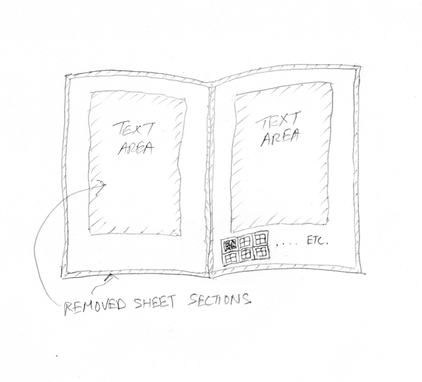
Each of these 3 × 3 cm “full squares” provided, in its interior, two 1 cm2 B (before-treatment) squares and two 1 cm2 A (after-treatment) squares. A 5 mm border protected the inner A and B squares during treatment, analysis, and sampling.
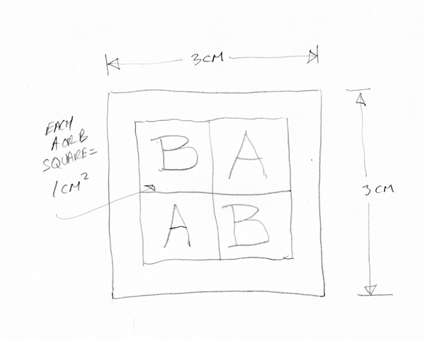
Each ICP-OES analysis required 100 mg of paper; therefore the number of full squares required depended on both the GSM (grams per square meter) of the paper and the number of treatments to be executed. Where print-free paper availability was limited, “half squares” were allowed; i.e., two 1 cm2 squares (one B, one A) instead of four; however, a 5 mm border was still required. Therefore a half square measured 2 × 3 cm.
Treatments
The treatments used on each specimen were as follows:
0. Control (same as before-treatment samples and tests)
1. Deionized water, cold
2. Deionized water, warm
3. Calcium hydroxide, low concentration (pH 8)
4. Calcium hydroxide, low concentration (pH 8), three times with intermediate drying
5. Calcium hydroxide, higher concentration (pH 9.5)
6. Calcium hydrogen carbonate (also known as calcium bicarbonate)
7. Calcium phytate / calcium hydrogen carbonate
Details on each treatment are provided in the appendix (below).
ICP destructive testing
Two before-treatment samples were taken from each specimen by sampling B squares from the XRF analysis locations until 100 mg was accumulated. This sampling routine was repeated on a fresh set of available full square B squares. Therefore for each specimen, two before-treatment ICP tests were performed and seven after-treatment ICP tests, or a total of nine tests per specimen. Nine specimens times nine ICP tests equals a total of eighty-one ICP analyses required during the experiment. Again, the number of 1 cm2 A or B squares in a sample for each ICP test varied depending on the GSM of the specimen. Due to the relocation of one of the coauthors while the experiment was in process, the ICP-OES work was accomplished in two laboratories, by two different technicians. Though not ideal, this was unavoidable. Details of the ICP-OES analytical procedures are available in the appendix (below).Specimen handling, sampling, and analysis
Terminology: “specimen” indicates the entire leaf or bifolio leaf; “sample” means the paper cut from the specimen for testing.
- Cotton gloves were used or the paper specimens were handled “on edge” for the duration of the experiment. Print-free paper was removed from each specimen using a diamond-bladed cutter and a self-healing pad, cutting a minimum of 5 mm away from any printed area or paper edge (Figure 1). Printed and edge pieces were saved in a Mylar envelope marked with the specimen number. All print-free pieces available for cutting into full squares were collected and stored in a separate Mylar envelope, again marked with the specimen number.
- Working on one specimen at a time, we cut out all possible full squares regardless of the total required, while avoiding any obvious bits of iron or other anomalies. From these full squares, we determined the average GSM for that specimen. We shuffled the entire set ten times to randomize the original location of the squares within the specimen sheet and removed the total number of full squares required for the experiment based on the GSM. For each specimen, there were seven groups of full squares; one group for each of the seven treatments. We reserved any extras in an envelope marked with the specimen number. Note: the B squares within each full square provided the before-treatment, or control-sample, material.
- Using the diamond cutter, a small triangle was cut from each full square roughly 2 mm from the upper-left corner, to serve as an orientation reference point. The specimen number was indicated by the same number of notches cut on the upper-right corner. On the lower-right corner, we cut notches equal to the treatment number. See Figure 3 (below).
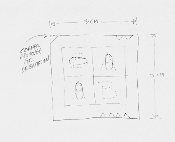
Figure 3. Full square notching and XRF analysis areas. - A series of XRF analyses of the CrBr (chromium and bromine) cup alone were done to establish a library of standard spectra. At the start of each new analysis day, a “cup only” scan was gathered and checked against this library to ensure that the instrument was operating properly. All XRF tests in this project were sixty seconds each. Between twenty and twenty-eight B-square before-treatment XRF tests were done on each specimen by randomly selecting the number of required full squares from the total available for the specimen. One XRF test was executed in the center of each upper-left B square. The analysis window on the Bruker instrument describes an ellipse of roughly 3 × 5 mm (Figure 3).
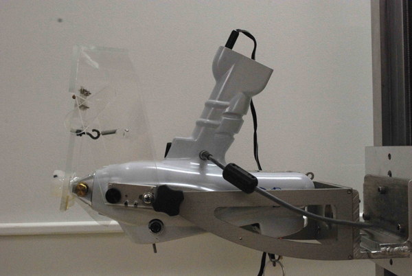
Figure 4. Bruker Tracer III-V handheld XRF instrument fitted with accessory. 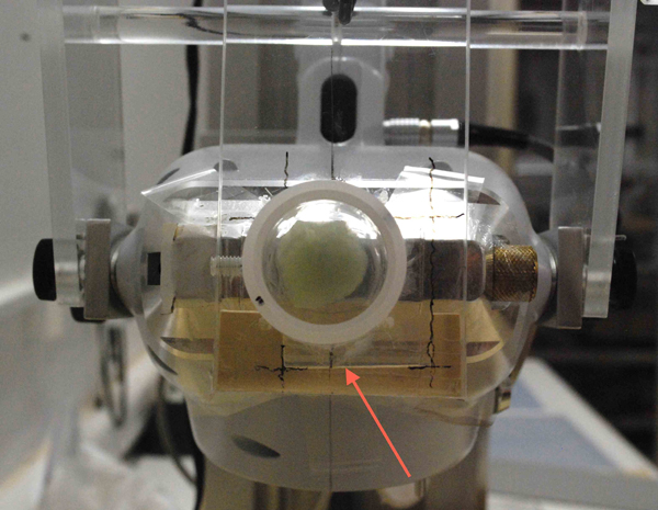
Figure 5. Red arrow indicates the shelf constructed for positioning full squares. - A specially made shelf was fitted to the XRF instrument’s acrylic accessory to ensure that the full square receiving analysis was positioned so the A or B square being tested was centered over the instrument nose (Figures 4 and 5). A thin Mylar strip on the lower portion of the face of the shelf kept the sample from falling during positioning and analysis. When all the spectra and the instrument performance were approved, the diamond cutter and a Mylar template were used to puncture the specimen against a self-healing pad to indicate the A and B square positions. We then sampled from each upper-left B square (from ten to fourteen full squares depending on the specimen’s GSM) at the center of the XRF analysis locations until 100 mg was accumulated. This was repeated, yielding two 100 mg samples for before-treatment ICP-OES analysis for that specimen. Note: the A squares were not tested with XRF at this time, as there were no corresponding ICP-OES analyses done on the A squares until after treatment. Again, see details of the ICP-OES analysis procedures in the appendix.
- Scheme for sample labels and XRF scan records:
2B1
2 = specimen number
B = before treatment
1 = sample number, 1 or 22A1
2 = specimen number
A = after treatment
1 = treatment number, 1–7 (all “after” samples are 1 sample each)Table 3
ICP SAMPLES
XRF RECORDS
Before treatment
2B1
2B1-1, 2B1-2, 2B1-3, etc.
2B2
3B1
3B2, etc.
After treatment
2A1
2A1-1, 2A1-2, 2A1-3, etc
2A2
2A3, etc.
- At the conclusion of the before-treatment XRF analyses and ICP sampling, all full squares were sent to Germany for aqueous treatments.
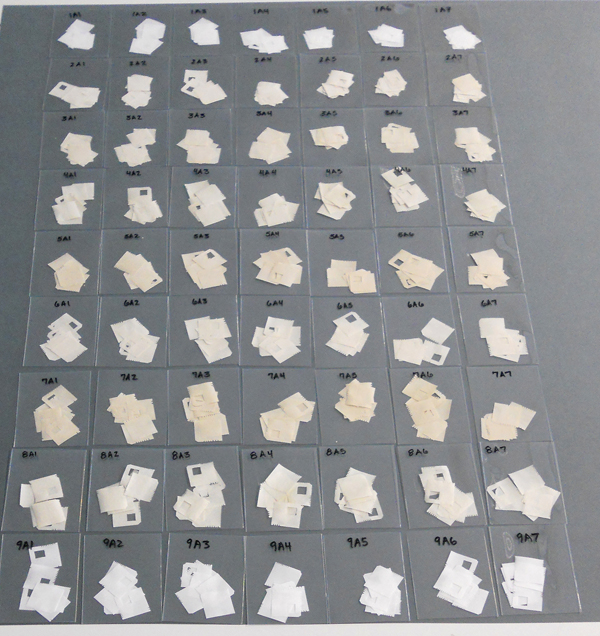
Figure 6. All samples after treatment in Germany. - Following treatments, all samples were returned to the University of Iowa Center for the Book for after-treatment XRF. One sixty-second XRF test was done on each A square (per Figure 3). All A square after-treatment sample material was then separated and delivered for ICP-OES analyses.
As mentioned, as a result of unanticipated personnel developments, the ICP-OES analyses were executed in two different laboratories, one at the Library of Congress’s Division of Research and Testing, the other at the University of Iowa’s Department of Geoscience.
IPC-OES data
Results of the ICP-OES analyses are shown in table 4. “BDL” stands for “beyond detection limit.” ICP-OES analyses were not completed on “NA” samples due to loss of sample material.
In the early stages of calibration work, it became clear that some of the ICP-OES data did not match the peaks in the XRF spectra associated with that sample. These were significant discrepancies that we later attributed to a number of possible sources of error during the experimental work. They included:
- sample mislabeling;
- seven workers in two countries handling eighty-one samples divided into 994 individual pieces of paper;
- stray compound or metal concentrations detected by one analysis method and not by the other; and
- use of two different laboratories for the ICP-OES analyses.
Samples with faulty data are highlighted in blue in table 4, but we elected not to include these data in our calibration work and plots.
Table 4
Sample |
Al ppm |
%RSD |
Ca ppm |
%RSD |
Cu ppm |
%RSD |
Fe ppm |
%RSD |
K ppm |
%RSD |
Mg ppm |
%RSD |
S ppm |
%RSD |
Zn ppm |
%RSD |
1B1 |
65 |
3.89 |
170 |
0.08 |
BDL |
18.41 |
7.5 |
9.57 |
56 |
34.6 |
12.5 |
0.25 |
90 |
0.46 |
1.5 |
1.26 |
1B2 |
580 |
1.23 |
1200 |
0.48 |
30 |
2.14 |
230 |
0.29 |
440 |
5.07 |
1000 |
0.36 |
580 |
0.38 |
15 |
0.36 |
1A1 |
50 |
11.81 |
110 |
0.74 |
BDL |
16.25 |
3.9 |
27 |
31 |
30.69 |
3.1 |
0.32 |
14 |
2.96 |
BDL |
7.17 |
1A2 |
60 |
13.62 |
190 |
0.31 |
BDL |
82.68 |
7.3 |
1.83 |
33 |
54.93 |
3.6 |
0.16 |
19 |
3.10 |
BDL |
1.61 |
1A3 |
59 |
15.4 |
2500 |
0.85 |
BDL |
21.45 |
5.5 |
19.26 |
9.1 |
125.3 |
11 |
0.11 |
66 |
1.49 |
BDL |
4.48 |
1A4 |
75 |
12.13 |
120 |
0.43 |
BDL |
58.39 |
8 |
3.17 |
33 |
37.43 |
15 |
0.72 |
28 |
1.25 |
1.1 |
0.38 |
1A5 |
40 |
12.01 |
63 |
0.34 |
BDL |
186.20 |
9.7 |
2.13 |
21 |
29.19 |
7.4 |
0.39 |
17 |
2.72 |
BDL |
3.81 |
1A6 |
58 |
0.89 |
3500 |
1.48 |
BDL |
64.86 |
8.7 |
20.40 |
25 |
57.04 |
14 |
0.54 |
86 |
2.94 |
BDL |
42.44 |
1A7 |
640 |
0.47 |
1200 |
0.70 |
27 |
5.65 |
330 |
0.18 |
76 |
29.54 |
1200 |
0.30 |
160 |
0.29 |
21 |
0.15 |
|
|
|
|
|
|
|
|
|
|
|
|
|
|
|
|
|
2B1 |
690 |
0.59 |
1900 |
0.36 |
48 |
2.57 |
350 |
0.21 |
680 |
0.96 |
1300 |
0.09 |
920 |
0.54 |
27 |
0.44 |
2B2 |
2400 |
0.04 |
3500 |
1.10 |
16 |
3.37 |
140 |
0.25 |
2300 |
0.34 |
380 |
0.23 |
6200 |
0.22 |
16 |
0.30 |
2A1 |
500 |
0.68 |
1300 |
0.29 |
24 |
1.60 |
300 |
0.30 |
61 |
19.03 |
950 |
0.36 |
120 |
0.42 |
19 |
0.35 |
2A2 |
|
|
|
|
|
|
|
|
|
|
|
|
|
|
|
|
2A3 |
360 |
2.08 |
1300 |
0.10 |
27 |
6.69 |
300 |
0.53 |
45 |
8.39 |
820 |
0.32 |
130 |
0.65 |
21 |
0.09 |
2A4 |
54 |
2.42 |
9 |
1.03 |
BDL |
90.6 |
1.3 |
25.64 |
5.5 |
587.7 |
1.4 |
1.50 |
3.1 |
14.45 |
BDL |
44.38 |
2A5 |
572 |
1.02 |
1138 |
0.42 |
25 |
2.00 |
264 |
0.76 |
39 |
2.19 |
1043 |
0.38 |
279 |
17.53 |
15 |
2.39 |
2A6 |
553 |
2.53 |
1451 |
1.01 |
24 |
2.88 |
273 |
1.67 |
33 |
1.85 |
1018 |
0.89 |
159 |
11.80 |
17 |
3.39 |
2A7 |
589 |
1.87 |
1673 |
0.74 |
33 |
1.24 |
281 |
1.63 |
39 |
2.65 |
1048 |
0.77 |
273 |
12.53 |
17 |
4.52 |
|
|
|
|
|
|
|
|
|
|
|
|
|
|
|
|
|
3B1 |
|
|
|
|
|
|
|
|
|
|
|
|
|
|
|
|
3B2 |
1700 |
1.343 |
3400 |
0.83 |
31 |
4.49 |
190 |
0.68 |
2100 |
0.58 |
400 |
0.5983 |
5000 |
0.1763 |
10 |
0.1903 |
3A1 |
1846 |
0.89 |
76 |
0.71 |
17 |
2.88 |
128 |
1.32 |
54 |
2.55 |
219 |
0.77 |
533 |
6.22 |
6.8 |
7.22 |
3A2 |
1800 |
1.15 |
60 |
0.42 |
10 |
2.20 |
123 |
3.25 |
43 |
1.08 |
221 |
0.44 |
454 |
7.04 |
7.2 |
8.97 |
3A3 |
2041 |
0.83 |
148 |
0.23 |
11 |
3.52 |
143 |
1.85 |
74 |
0.92 |
226 |
0.17 |
453 |
5.38 |
10.7 |
4.71 |
3A4 |
2026 |
1.36 |
178 |
0.45 |
12 |
2.18 |
134 |
3.90 |
37 |
4.16 |
219 |
0.51 |
348 |
4.68 |
7.0 |
2.66 |
3A5 |
2110 |
1.15 |
335 |
0.39 |
14 |
2.57 |
131 |
2.24 |
66 |
0.78 |
219 |
0.49 |
428 |
5.23 |
7.7 |
4.38 |
3A6 |
2182 |
1.32 |
625 |
0.73 |
13 |
1.22 |
130 |
2.65 |
64 |
0.91 |
222 |
0.70 |
254 |
9.73 |
8.5 |
3.99 |
3A7 |
2029 |
0.15 |
1159 |
0.55 |
20 |
1.49 |
130 |
1.36 |
51 |
1.11 |
237 |
0.49 |
275 |
3.95 |
20.9 |
1.07 |
|
|
|
|
|
|
|
|
|
|
|
|
|
|
|
|
|
4B1 |
2100 |
0.41 |
3700 |
0.41 |
37 |
7.91 |
230 |
0.08 |
2500 |
1.46 |
500 |
0.22 |
5500 |
0.49 |
13 |
0.82 |
4B2 |
1500 |
0.65 |
4000 |
0.56 |
7.7 |
5.45 |
250 |
0.60 |
1700 |
0.41 |
480 |
0.31 |
6000 |
0.25 |
10 |
0.14 |
4A1 |
1522 |
0.58 |
206 |
0.14 |
24 |
1.02 |
205 |
2.09 |
34 |
2.98 |
224 |
0.58 |
437 |
6.40 |
9.0 |
2.83 |
4A2 |
1510 |
0.95 |
147 |
0.33 |
23 |
1.31 |
203 |
2.77 |
29 |
2.37 |
223 |
0.41 |
325 |
8.92 |
8.6 |
6.35 |
4A3 |
1640 |
0.68 |
354 |
0.48 |
23 |
0.67 |
217 |
1.38 |
36 |
1.28 |
230 |
0.73 |
409 |
2.69 |
7.5 |
2.26 |
4A4 |
1621 |
0.99 |
363 |
0.16 |
23 |
2.16 |
208 |
2.28 |
16 |
3.17 |
221 |
0.20 |
401 |
8.85 |
8.0 |
2.95 |
4A5 |
1744 |
1.26 |
552 |
0.25 |
24 |
2.80 |
209 |
2.02 |
40 |
0.98 |
230 |
0.26 |
541 |
1.70 |
7.5 |
4.05 |
4A6 |
1664 |
1.39 |
1054 |
0.47 |
26 |
1.44 |
214 |
3.07 |
41 |
2.15 |
234 |
0.78 |
284 |
5.40 |
11.4 |
4.38 |
4A7 |
1612 |
1.78 |
1467 |
0.36 |
27 |
1.77 |
198 |
1.90 |
22 |
3.10 |
240 |
0.62 |
473 |
8.07 |
8.3 |
4.44 |
|
|
|
|
|
|
|
|
|
|
|
|
|
|
|
|
|
5B1 |
1400 |
0.57 |
3700 |
0.35 |
6.9 |
18.68 |
250 |
0.42 |
1700 |
0.49 |
440 |
0.33 |
6000 |
0.26 |
9.7 |
0.33 |
5B2 |
1000 |
1.04 |
1400 |
0.92 |
8.1 |
12.76 |
200 |
0.79 |
1700 |
0.45 |
370 |
0.48 |
2700 |
0.12 |
8.7 |
0.36 |
5A1 |
1041 |
0.99 |
177 |
0.79 |
5.11 |
2.75 |
206 |
4.26 |
32 |
2.55 |
195 |
0.82 |
362 |
7.45 |
3.8 |
5.04 |
5A2 |
1021 |
1.46 |
137 |
1.00 |
5.70 |
2.75 |
211 |
1.70 |
26 |
4.21 |
201 |
0.84 |
472 |
13.36 |
5.1 |
4.78 |
5A3 |
1060 |
2.20 |
304 |
0.46 |
4.40 |
2.81 |
212 |
2.61 |
37 |
2.12 |
197 |
0.75 |
306 |
7.84 |
4.3 |
3.47 |
5A4 |
1031 |
1.32 |
345 |
0.48 |
4.91 |
2.01 |
210 |
4.32 |
18 |
2.50 |
194 |
0.42 |
260 |
5.98 |
5.2 |
4.58 |
5A5 |
1092 |
1.14 |
495 |
0.51 |
6.53 |
4.32 |
211 |
2.31 |
39 |
2.50 |
194 |
0.35 |
277 |
4.10 |
4.5 |
2.14 |
5A6 |
1079 |
1.42 |
702 |
0.34 |
5.69 |
5.68 |
219 |
1.56 |
42 |
2.53 |
190 |
0.59 |
262 |
9.00 |
7.2 |
7.41 |
5A7 |
1146 |
1.20 |
1368 |
0.58 |
14.74 |
2.62 |
214 |
1.58 |
28 |
1.21 |
203 |
0.75 |
495 |
6.65 |
6.2 |
5.65 |
|
|
|
|
|
|
|
|
|
|
|
|
|
|
|
|
|
6B1 |
1500 |
0.05 |
1800 |
0.66 |
12 |
17.95 |
270 |
0.79 |
2400 |
1.23 |
660 |
0.62 |
4000 |
0.46 |
13 |
0.56 |
6B2 |
2100 |
0.68 |
850 |
0.63 |
24 |
6.46 |
240 |
0.17 |
3500 |
0.54 |
280 |
0.13 |
4000 |
1.18 |
8.6 |
1.06 |
6A1 |
1013 |
1.16 |
196 |
0.45 |
16.72 |
3.62 |
208 |
3.25 |
6 |
1.66 |
271 |
0.57 |
385 |
2.98 |
8.3 |
0.75 |
6A2 |
972 |
1.73 |
149 |
0.44 |
5.81 |
3.41 |
208 |
1.24 |
42 |
1.53 |
194 |
0.47 |
207 |
13.13 |
9.4 |
6.26 |
6A3 |
963 |
1.28 |
356 |
0.32 |
7.84 |
2.23 |
220 |
3.11 |
52 |
1.33 |
206 |
0.48 |
157 |
10.31 |
9.7 |
4.34 |
6A4 |
994 |
1.85 |
427 |
0.12 |
5.71 |
3.85 |
201 |
3.23 |
25 |
1.61 |
187 |
0.27 |
382 |
14.43 |
6.0 |
8.11 |
6A5 |
976 |
2.03 |
604 |
0.32 |
5.28 |
7.18 |
214 |
2.97 |
49 |
1.45 |
198 |
0.23 |
277 |
10.61 |
7.4 |
5.28 |
6A6 |
1030 |
2.09 |
1019 |
0.61 |
6.43 |
5.23 |
216 |
1.37 |
49 |
1.06 |
191 |
0.97 |
199 |
12.68 |
6.7 |
4.52 |
6A7 |
980 |
1.65 |
1025 |
0.44 |
9.41 |
1.88 |
220 |
1.19 |
24 |
4.99 |
186 |
0.47 |
259 |
6.96 |
10.5 |
5.15 |
|
|
|
|
|
|
|
|
|
|
|
|
|
|
|
|
|
7B1 |
110 |
8.78 |
3000 |
0.82 |
3.5 |
57.71 |
16 |
4.07 |
260 |
6.93 |
150 |
0.12 |
900 |
0.06 |
4.3 |
0.97 |
7B2 |
|
|
|
|
|
|
|
|
|
|
|
|
|
|
|
|
7A1 |
1297 |
0.76 |
82 |
1.23 |
15.22 |
0.73 |
200 |
2.41 |
81 |
0.69 |
122 |
0.61 |
299 |
10.54 |
3.0 |
7.69 |
7A2 |
1243 |
1.63 |
70 |
0.18 |
14.54 |
2.23 |
194 |
1.86 |
78 |
1.58 |
119 |
0.35 |
508 |
13.32 |
2.9 |
5.10 |
7A3 |
1375 |
0.77 |
204 |
0.36 |
19.11 |
0.90 |
204 |
2.02 |
84 |
0.85 |
122 |
0.52 |
296 |
3.11 |
2.8 |
6.20 |
7A4 |
1327 |
0.74 |
262 |
0.48 |
15.35 |
1.03 |
187 |
3.03 |
62 |
0.82 |
121 |
0.61 |
289 |
8.48 |
3.5 |
7.16 |
7A5 |
1454 |
1.26 |
432 |
0.59 |
19.04 |
1.36 |
205 |
0.75 |
101 |
0.76 |
126 |
0.68 |
257 |
7.84 |
7.4 |
14.93 |
7A6 |
1369 |
0.82 |
662 |
0.58 |
18.62 |
1.17 |
190 |
4.18 |
91 |
0.84 |
123 |
0.40 |
317 |
7.10 |
3.0 |
9.50 |
7A7 |
1473 |
1.18 |
1043 |
0.56 |
25.31 |
1.31 |
192 |
1.64 |
65 |
1.14 |
139 |
0.50 |
247 |
9.84 |
3.0 |
4.77 |
|
|
|
|
|
|
|
|
|
|
|
|
|
|
|
|
|
8B1 |
150 |
2.469 |
4500 |
1.29 |
4.8 |
14.13 |
21 |
5.27 |
300 |
1.94 |
220 |
0.59 |
880 |
0.45 |
4.6 |
0.16 |
8B2 |
64 |
6.304 |
250 |
0.79 |
BDL |
57.92 |
5.3 |
14.97 |
21 |
109.40 |
27 |
0.88 |
350 |
0.58 |
1.8 |
1.44 |
8A1 |
112 |
2.30 |
6385 |
0.87 |
5.43 |
4.70 |
21 |
9.69 |
6 |
7.68 |
100 |
0.81 |
339 |
7.17 |
3.7 |
16.54 |
8A2 |
90 |
6.37 |
6258 |
0.51 |
5.57 |
2.92 |
22 |
11.06 |
8 |
2.79 |
93 |
0.49 |
535 |
17.41 |
3.2 |
14.01 |
8A3 |
126 |
9.72 |
6998 |
0.48 |
3.47 |
2.12 |
25 |
7.06 |
6 |
6.38 |
101 |
0.56 |
423 |
9.56 |
2.0 |
5.33 |
8A4 |
101 |
2.19 |
6599 |
0.46 |
4.24 |
2.32 |
27 |
8.45 |
6 |
11.37 |
82 |
0.62 |
217 |
4.07 |
5.3 |
6.14 |
8A5 |
81 |
2.98 |
7738 |
0.42 |
4.81 |
2.60 |
21 |
7.57 |
11 |
1.90 |
102 |
0.58 |
282 |
6.14 |
3.0 |
9.64 |
8A6 |
139 |
5.56 |
4171 |
0.75 |
10.45 |
3.74 |
33 |
5.90 |
15 |
2.76 |
64 |
0.78 |
187 |
8.76 |
7.5 |
7.27 |
8A7 |
139 |
2.36 |
6240 |
0.14 |
13.45 |
1.53 |
22 |
6.49 |
4 |
4.87 |
99 |
0.31 |
415 |
6.71 |
3.0 |
6.38 |
|
|
|
|
|
|
|
|
|
|
|
|
|
|
|
|
|
9B1 |
58 |
11.04 |
240 |
0.25 |
BDL |
47.33 |
7.7 |
8.14 |
18 |
85.95 |
24 |
0.28 |
330 |
0.30 |
BDL |
3.40 |
9B2 |
58 |
7.954 |
140 |
0.42 |
BDL |
36.73 |
7.3 |
3.30 |
BDL |
473.3 |
4.1 |
0.17 |
19 |
2.20 |
BDL |
2.79 |
9A1 |
12 |
34.78 |
103 |
0.72 |
BDL |
15.27 |
4.4 |
13.47 |
1 |
14.74 |
13 |
0.54 |
246 |
2.69 |
BDL |
16.72 |
9A2 |
12 |
14.01 |
70 |
0.77 |
1.77 |
2.47 |
2.1 |
21.40 |
2 |
7.33 |
13 |
1.68 |
373 |
6.68 |
BDL |
13.72 |
9A3 |
29 |
21.99 |
203 |
0.55 |
BDL |
7.57 |
BDL |
43.64 |
2 |
7.71 |
7 |
0.51 |
280 |
3.50 |
BDL |
23.99 |
9A4 |
23 |
13.91 |
192 |
0.50 |
48.25 |
1.78 |
0.3 |
28.56 |
5 |
10.01 |
4 |
1.16 |
250 |
6.41 |
BDL |
29.33 |
9A5 |
17 |
34.35 |
281 |
0.37 |
BDL |
13.32 |
2.0 |
16.53 |
2 |
13.77 |
5 |
0.60 |
268 |
8.50 |
BDL |
4.15 |
9A6 |
20 |
18.17 |
945 |
0.27 |
0.29 |
7.10 |
BDL |
22.90 |
1 |
8.35 |
8 |
1.18 |
256 |
8.40 |
BDL |
25.25 |
9A7 |
11 |
15.03 |
600 |
0.35 |
3.60 |
2.29 |
1.0 |
20.61 |
4 |
9.21 |
11 |
0.96 |
239 |
8.57 |
BDL |
17.63 |
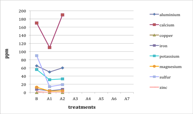
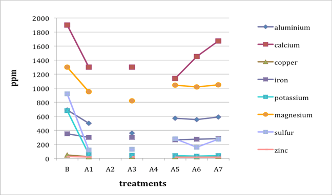
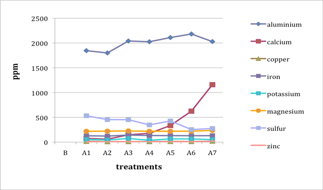
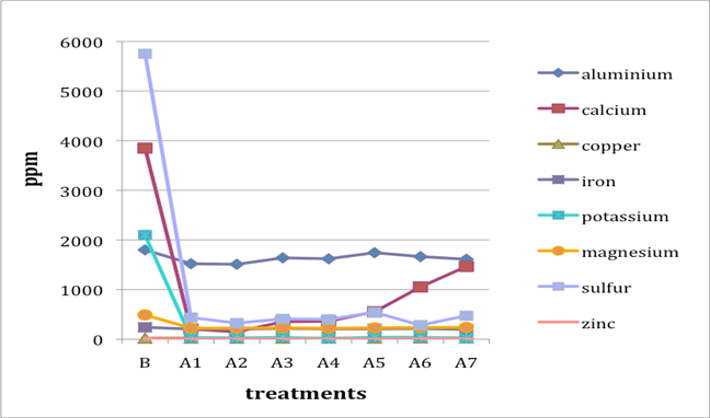
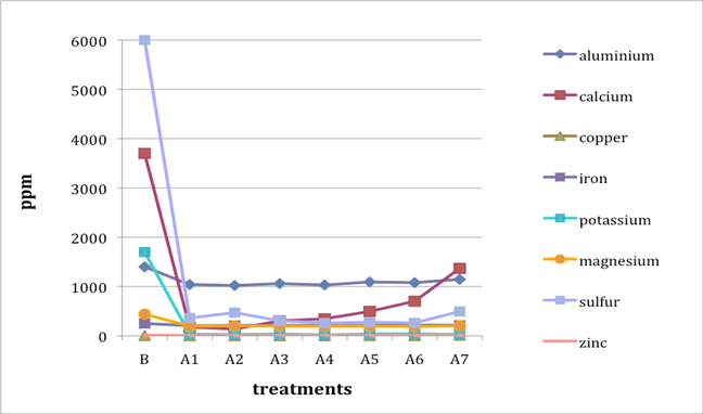
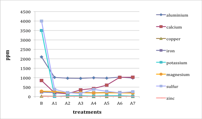
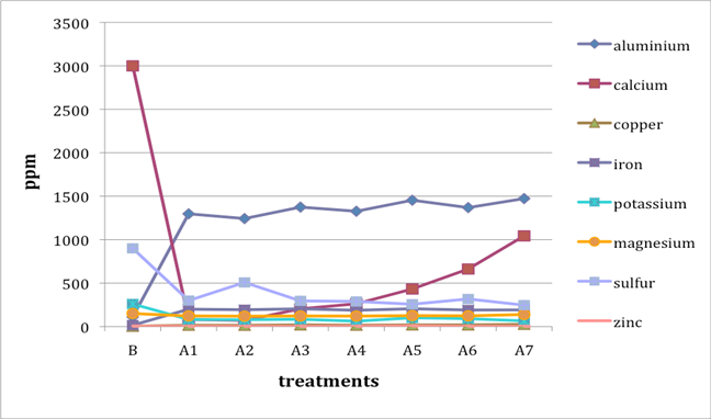
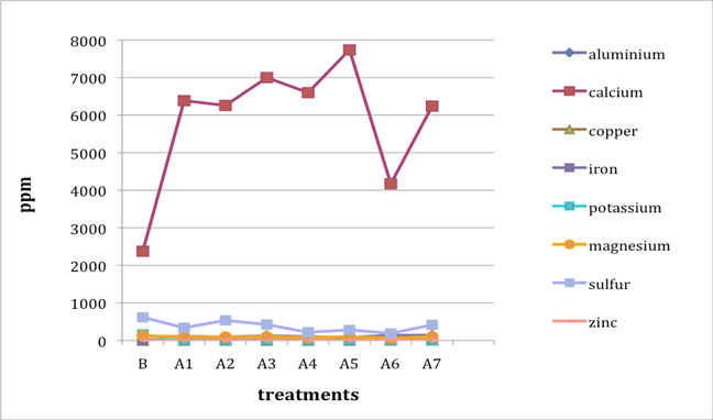
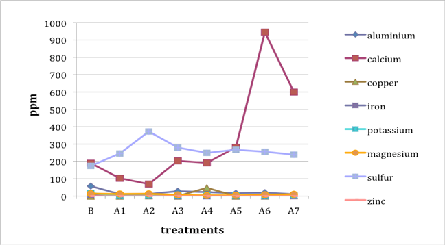
Observed changes during treatment
When two B (before-treatment) samples were tested, the results were averaged for plotting purposes. Results for Cu and Zn were either BDL (beyond detection limit) or only present in single or double-digit concentrations. They are included in the plots despite the low concentrations observed. See the discussion section below for an analysis of the results. Suspect data shown in blue in table 4 (above) was not included in the plots. The vertical axis in all plots shows concentration in ppm; the horizontal axis shows first the before-treatment result followed by the results after each treatment type. The horizontal axis therefore does not represent steps in an extended treatment regime; rather it shows the results following independent treatments.
The treatments are listed again (below) for ease of reference. B (before treatment) and A (after treatment) have been added to the respective numbers to correspond to the plots that follow.
B0. Control (same as before-treatment samples and tests)
A1. Deionized water, cold
A2. Deionized water, warm
A3. Calcium hydroxide, low concentration (pH 8)
A4. Calcium hydroxide, low concentration (pH 8), three times with intermediate drying
A5. Calcium hydroxide, higher concentration (pH 9.5)
A6. Calcium hydrogen carbonate (also known as calcium bicarbonate)
A7. Calcium phytate / calcium hydrogen carbonate
Calibration results
Plot 1 (below) shows the calibration fit for Ca.
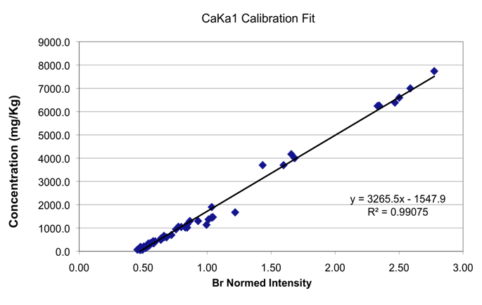
R2 values for fits from our earlier original calibration and the new current calibration are shown in table 5 below.
Table 5
| Element | Original R2 fit | Approximate range mg/kg | New R2 fit | Approximate range mg/kg |
|---|---|---|---|---|
S |
.9272 |
180–3,970 |
.9516 |
14–6,000 |
K |
.9237 |
70–1,730 |
.9586 |
0–2,500 |
Ca |
.9534 |
680–24,000 |
.9908 |
60–7,738 |
Fe |
.8881 |
127–555 |
.981 |
0–350 |
Selecting a result near 1,000 ppm, or the highest result, and comparing the propagated error (2 × standard deviation) as done in table 6 (below) shows similar results for all elements but Fe. The R2 value in table 5 gives an idea of the accuracy of the fit, and for all but Fe at most one interference correction was used. However, in the original calibration five corrections were used for Fe. The uncorrected fit had an R2 value of 0.54, and it took five corrections to get the R2 up to the 0.89 value listed in table 5.
In comparison, the uncorrected R2 value for Fe in the new calibration was 0.94 before adding one slope-type correction based on the thickness/density value. There are at least two possible explanations, and both likely play a part. The first is that scanning the exact spot used for the ICP testing is more critical for Fe, either due to variations in the iron concentrations that may result from contamination during handling or because iron is a very common element and its presence varies significantly in the manufacturing process. The other possibility is that Fe Ka1 fluorescence has the highest energy of the elements calibrated and hence can be “seen” deeper into the sample. The other elements would reach an effective infinite thickness sooner than Fe, and given that in the new calibration our thickness/density number was used to improve the R2 value from 0.94 to 0.98, the thickness/density does seem to be important for the Fe calibration. The thickness/density data was not nearly as useful in the original calibration, perhaps because other variations obscured the effect.
Table 6: Original and New Calibrations Compared
|
Original calibration | New calibration | ||||
|---|---|---|---|---|---|---|
|
Fit Conc. |
2stdev prop. error | >
|
Fit Conc. |
2stdev prop. error |
|
S |
1,082 |
100 |
9.24% |
1246 |
121 |
9.71% |
K |
956 |
96 |
10.04% |
1592 |
133 |
8.35% |
Ca |
1,046 |
70 |
6.69% |
1160 |
75 |
6.47% |
Fe |
869 |
195 |
22.44% |
297 |
36 |
12.12% |
In the first calibration, several samples excluded from the calibration were used to test for accuracy and precision. These same samples were still available for the newer calibration and similar tests were done. The results were similar but on average better with the new calibration. The average bias went from -6.6% in the original calibrations to 2.8% in the new calibrations. The average precision was slightly improved, but given that the same instrument and conditions were used, the change is from the exact corrections used, introducing fewer variations. Table 7 provides more detail. The ICP results were treated as the accepted values. In addition, for sample D5, tests were also done where the CrBr cup was lifted, the specimen moved to a new position, and the analysis repeated. It was expected that the precision would be worse when the cup was lifted and the artifact repositioned, and this increase gives an indication of the variation across the paper.
Table 7: Accuracy and Precision Calculation Results
Accepted
ICP |
S |
K |
Ca |
Fe |
D5-lift |
3220 |
1260 |
1140 |
106 |
D5 |
3220 |
1260 |
1140 |
106 |
D16 |
2620 |
1670 |
759 |
188 |
L2 |
665 |
468 |
19900 |
302 |
L19 |
361 |
282 |
5280 |
291 |
XRF
Bias |
S Ka1 |
K Ka1 |
CaKa1 |
FeKa1 |
D5-lift |
36.69% |
31.51% |
-13.40% |
18.55% |
D5 |
41.35% |
10.44% |
-8.36% |
15.31% |
D16 |
31.17% |
12.41% |
6.82% |
-4.60% |
L2 |
-71.30% |
-43.75% |
-14.91% |
-9.47% |
L19 |
60.63% |
30.79% |
5.41% |
-17.59% |
Average |
15.46% |
2.47% |
-2.76% |
-4.09% |
Previous calibration |
|
|
|
|
D5 |
0.74% |
22.49% |
-26.61% |
-1.11% |
D16 |
-17.24% |
-0.98% |
-15.89% |
21.14% |
L2 |
13.75% |
17.94% |
-10.82% |
2.07% |
L19 |
-62.81% |
-40.16% |
2.17% |
-11.12% |
Average |
-16.39% |
-0.18% |
-12.79% |
2.75% |
STDEV |
S Ka1 |
K Ka1 |
CaKa1 |
FeKa1 |
D5-lift |
9.52% |
22.59% |
14.59% |
20.24% |
D5 |
4.74% |
6.90% |
5.49% |
13.28% |
D16 |
6.57% |
5.32% |
10.16% |
5.60% |
L2 |
21.75% |
38.47% |
2.61% |
8.67% |
L19 |
18.46% |
22.96% |
3.19% |
7.03% |
Average |
12.88% |
18.42% |
5.36% |
8.64% |
Previous calibration |
|
|
|
|
D5 |
8.04% |
8.46% |
6.53% |
19.85% |
D16 |
5.53% |
4.93% |
9.34% |
8.01% |
L2 |
16.86% |
16.32% |
2.24% |
4.23% |
L19 |
64.49% |
62.46% |
4.77% |
7.22% |
Average |
23.73% |
23.04% |
5.72% |
9.83% |
Limits of detection
The limit of detection (LOD) in this work and in most XRF research is the lowest concentration that is likely to be detected. In other fields LOD is considered to be, more generally, the lowest level that will be detected. Often three standard deviations are used in defining the LOD, occasionally two. The XRF community takes a somewhat different approach. Additional detail is provided in the appendix.
The limits of detection shown in table 8 (below) were calculated from the sample with the lowest and highest count rates in the calibration data for a given element. A simple line was used as a calibration, and the counts at zero concentration were determined from this line. The product of the slope of the line and three times the square root of the counts at zero concentration was then used as the LOD. This calculation was for the instrument, and not for the calibration, hence the better LOD found in the current data set is likely due to a difference between the paper used for the instrument LOD tests and that used for the calibrations. Results appear under the heading of “Est. inst.” for estimated LOD of the instrument only.
Table 8: Limits of Detection for Instrument Only
|
Scan time (sec.) |
Scan time (sec.) |
Scan time (sec.) |
Scan time (sec.) |
Scan time (sec.) |
|
LOD(ppm) |
30 |
60 |
120 |
180 |
300 |
Est. inst. |
Al Ka1 |
1089 |
770 |
544 |
444 |
344 |
221 |
S Ka1 |
195 |
138 |
97 |
80 |
62 |
39 |
K Ka1 |
132 |
94 |
66 |
54 |
42 |
27 |
Ca Ka1 |
143 |
101 |
72 |
59 |
45 |
29 |
Fe Ka1 |
32 |
23 |
16 |
13 |
10 |
7 |
An easy way to estimate the LOD for the instrument with the calibration is to simply find a calibration sample with zero concentration and run it through the calibration, which calculates the propagated error. Three standard deviations of this propagated error are the LOD in that sample. We did not have zero concentrations for all elements, but we did have very low concentrations for all elements in selected samples, and we felt the propagated error for concentrations near the detection limit should provide a good estimate of the LOD. Table 9 shows the results of such a test, along with the results for a 730-second LOD using the method described for table 8.
Table 9: Limits of Detection for Instrument with Calibration
|
Propagated error as LOD |
||
730 sec. |
mg/kg |
Sample |
3-sigma |
Al Ka1 |
11.1 |
9A7 |
258 |
S Ka1 |
14.0 |
1A1 |
116 |
K Ka1 |
0.0 |
9B2 |
110 |
Ca Ka1 |
59.6 |
3A2 |
69 |
Fe Ka1 |
0.0 |
9A3 |
18 |
In summary, we hoped the accuracy in this new calibration would improve because we took care to do destructive ICP-OES analyses only on sample material from the exact same location where XRF scans were done. We also based the experiment on a limited number of historical specimens and controls subjected to the same aqueous treatments. The results, however, were similar to those in the original calibration for Ca, K, and S, while the results for Fe were improved.
For Ca, K, and S, we believe the new calibration allows us to again estimate ppm concentrations with a precision of +/-20% at a 90% confidence level when concentrations are near 1,000 mg/kg (ppm). For Fe, our precision improved from +/-20% to 18% at a 90% confidence level when concentrations are near 300 mg/kg. These values are rough guidelines. Table 7 includes the standard deviations for several samples along with their concentrations, allowing more exact precision estimates by specimen and element. For reference, one standard deviation has a confidence interval of 68.3%; two standard deviations have a confidence interval of 95.5%. The 90% confidence interval corresponds to about 1.7 standard deviations.
Discussion
Changes during treatment
We note that with only two exceptions the concentrations of all elements in all the historical specimens (specimens 2–7) remained steady or dropped as a result of exposure to either cool or warm water (treatments 1 or 2). One exception was Fe and Al for specimen 7. There were no known sources of Al and Fe in the wash water. If the single B (before-treatment) sample data for specimen 7 is correct, another source of Al or Fe contamination may explain the increase in Fe and Al. The other exception is the result for specimen 2, treatment 2, for which the data was faulty and therefore not included in the plot.
An additional trend of note is that treatments A4–A7 result in increasing Ca pickup when the results are compared with those from the other treatments in the series. We lack data for specimen 2 to confirm this trend for all the historical specimens. However, even the highest Ca deposits (treatment 7) do not equal the original Ca levels found in the B samples, with the single exception of specimen 6. The result for specimen 3 is unknown due to excluded suspect data for the B samples.
Interestingly, Al, which we consider indicative of alum concentration, remains surprisingly flat across the series of treatments. In other words, much of the original Al appears to remain in the specimen, regardless of treatment. S and K may also be indicative of alum concentration, but they are not present at the levels observed for Al. Full results for specimen 2 are missing due to excluded suspect data.
The behavior of the control specimens (1, 8, and 9) is anomalous when compared with that of the historical specimens. For specimen 8, lime (calcium hydroxide) was used in cooking the fiber. In specimens 8 and 9, a high-Ca-content (4,000 ppm) photo gelatin was used for sizing, and for specimen 8, alum was added to the gelatin solution at a rate of 1% potassium aluminum sulfate on dry gelatin weight. These new, rather than aged, components in the controls may explain some of the erratic results observed in the control specimens. Much of the data for specimen 1, Whatman Grade 4 Chr paper, unsized, is missing due to excluded suspect data.
New calibration
We consider the level of precision described under the results (above) to be too low for monitoring the concentration of Ca, Fe, K, and S in single items during treatment but adequate for collections surveys where condition reports on hundreds of items are needed.
Conclusions
A total of 994 XRF and 81 ICP-OES analyses were executed on six historical papers and three controls before and after seven aqueous treatments.
The ICP-OES data showed the following trends of note:
- In five of the six historical specimens, Ca concentration increased with exposure to more alkaline alkalizing solutions; however, in four of the six, Ca concentration dropped from the before-treatment levels and never returned to the original levels, even when exposed to the highest concentrations of alkalizing compounds.
- 2. In five of the six the historical specimens, after an initial drop in Al concentration from before-treatment levels, Al concentration was surprisingly unaffected by different treatments. The exception was specimen 7, for which the data showed an actual increase over the before-treatment concentration, a response that was unexpected and is perhaps related to faulty data.
If we assume the Ca in the historical specimens is tied to desirable alkalizing compounds and Al is tied to residual alum in the paper, these trends suggest aqueous treatment may be removing more and replacing less Ca than desired and also removing less Al than desired. These trends deserve additional research attention. We wish to emphasize once again, however, that the historical paper specimens used in this work were chosen for their large print-free areas and not for their apparent need for aqueous treatment.
For Ca, K, and S, we believe the new calibration allows us to estimate ppm concentrations with a precision of +/-20% at a 90% confidence level when concentrations are near 1,000 mg/kg (ppm). For Fe, our precision improved from +/-20% to +/-18% at a 90% confidence level when concentrations are near 300 mg/kg. These values are rough guidelines.
Acknowledgements
Special thanks to Jay Thomas, who accomplished fifty-two of the eighty-one ICP-OES analyses. Research assistants Heather Wetzel and Lee Marchalonis executed many of the XRF analyses and the sample-weighing work prior to the ICP-OES analyses.
Suppliers
Diamond cutter
A Meyco diamond cutter with a 2 mm wide blade set perpendicular to the handle was used in this research; however, the original supplier is unknown. Meyco diamond scalpels are available from http://www.emsdiasum.com/microscopy/products/tweezers/diamond_scapel.aspx.
Paper specimens
All paper specimens used in this study were drawn from the UICB paper-specimen research collection. Contact principal investigator T. Barrett for details.
APPENDIX
Wet Treatment Details
Wet treatment 1: deionized water, cold
Chemicals used: cold deionized water (15–21°C)
Duration of washing: one hour
Procedure:
The deionzed water was drawn from a Herco Wassertechnik water-purification system. The water was kept in a refrigerator for about two hours, to reach a temperature of 15°C. The paper samples were put in separate trays made of Melinex in a bath of 200 ml of the cold deionized water. After one hour, the bath temperature was measured again, and it had adapted to the room temperature of about 21°C. The paper samples were then put on a screen to air-dry.
Tests:
Water hardness, amount of Mg and Ca ions, and the pH of the baths were measured before and after treatment. All measurements were performed on bath number 5 and assumed to be the same for all nine baths. Water hardness was measured using a VISOCOLOR Total Hardness H 20 Fcomplexometric titration test kit. The amount of Mg ions was measured by colorimetric determintion with Mann and Yoe’s magnesium reagent (xylidyl blue reagent) supplied as Aquamerck magnesiumfrom Merck. The amount of Ca ions was determined with test strips and reagents for the detection and semiquantification of Ca ions using Merckoquant calcium test stripsfrom Merck. The pH was measured with a precision laboratory pH meter by Präcitronic as well as a compact waterproof Twin pH meter by Horiba.
“Before” 5A1 |
“After” 5A1 |
a. water hardness: 0 mmol, < 0.5 °d |
a. water hardness: 0.3 mmol, 1.75 °d |
Wet treatment 2: deionized water, warm
Chemicals
used: warm deionized water (34°C)
Duration of
washing: one hour
Procedure:
Two liters of deionized water from the Herco Wassertechnik system was heated on a hot plate to raise it from a room temperature of 21°C to about 38°C. The paper samples were put in separate trays made of Melinex, in a bath of 200 ml of warm (34°C) deionized water. All nine sample baths were put in a hot-water bath to keep the temperature in the Melinex trays stable. After one hour, the paper samples were put on a screen to air-dry.
Tests:
“Before” 5A2 |
“After” 5A2 |
a. water hardness: 0.2 mmol, 1 °d |
a. water hardness: 0.9 mmol, 5 °d |
Wet treatment 3: calcium hydroxide, low concentration (pH 8)
Chemicals
used: calcium hydroxide, deionized water
Duration of
washing: one hour
Procedure:
For the conditioning of the calcium hydroxide bath, saturated Ca(OH)2 with a pH of 12.75 was added to 10 liters of deionized water to prepare the solutions for wet treatments 3, 4 ,and 5 at one time. After adjusting to a pH of 8, 1.8 liters was taken to fill nine baths of 200 ml each. The samples were put into the calcium hydroxide baths for 1 hour and afterward taken out and put on a screen to air-dry.
Tests:
“Before” 5A3 |
“After” 5A3 |
a. water hardness: 0.2 mmol, 1 °d |
a. water hardness: 0.4 mmol, 2 °d |
Wet treatment 4: calcium hydroxide, low concentration (pH 8), three times with intermediate drying
Chemicals
used: calcium hydroxide, deionized water
Duration of
washing: one hour (without intermediate drying)
Procedure:
The already prepared calcium hydroxide solution with a pH of 8 was added to the nine Melinex trays—again 200 ml for each bath. The samples were put into the calcium hydroxide baths for twenty minutes, taken out, and left to air-dry on a screen. For the second bath, the pH was once again adjusted to 8, and the dried samples received a second wet treatment. The treatment was repeated for a third time, again with an adjusted pH of 8. After one hour of washing, the samples were put on a screen to air-dry.
Tests:
“Before” 5A4 |
“After” 5A4-1 |
a. water hardness: 0.2 mmol, 1 °d |
a. water hardness: 0.4 mmol, 2 °d |
“After” 5A4-2 |
“After” 5A4-3 |
a. water hardness: 0.2 mmol, 1 °d |
a. water hardness: 0.2 mmol, 1 °d |
Wet treatment 5: calcium hydroxide, higher concentration (pH 9.5)
Chemicals
used: calcium hydroxide, deionized water
Duration of
washing: one hour
Procedure:
A total of 1.8 liters of the already prepared calcium hydroxide solution with a pH of 8 was conditioned to pH 9.5 by adding more of the saturated Ca(OH)2 solution (pH 12.75). The paper samples were put in Melinex trays containing 200 ml of the calcium hydroxide solution. After one hour of washing, the samples were taken out and put on a screen to air-dry.
Tests:
“Before” 5A5 |
“After” 5A5 |
a. water hardness: 0.5 mmol, 3 °d |
a. water hardness: 0.5 mmol, 2.75 °d |
Wet treatment 6: calcium hydrogen carbonate
Chemicals
used: calcium carbonate, deionized water
Duration of
washing: one hour
Procedure:
One gram of CaCO3 was added to two liters of deionized water and stirred for one minute. The dispersion was carbonated with a SodaStream soda maker. The prepared calcium hydrogen carbonate solution was kept in a refrigerator at 15°C until the wet treatment baths were prepared. The solution was added to the nine Melinex trays and the paper samples added to the baths. After one hour of washing, the samples were taken out and put on a screen to air-dry.
Tests:
“Before” 5A6 |
“After” 5A6 |
a. water hardness: could not be determined |
a. water hardness: could not be determined |
Wet treatment 7: calcium phytate, calcium hydrogen carbonate
Chemicals
used: phytic acid, calcium carbonate, deionized water
Duration of
washing: one hour
Procedure:
To prepare the phytate solution, 0.88 g of CaCO3 was dissolved in 5.76 g of phytic acid. The formation of foam was observed. The mixture was added to two liters of deionized water. The pH was adjusted to 5.3 using ammonia. The paper samples received a wet treatment in the phytate solution for thirty minutes. Afterward the paper samples were transferred into baths of calcium hydrogen carbonate, where they remained for another thirty minutes. The samples received no intermediate drying. The calcium hydrogen carbonate solution was prepared as described for wet treatment 6. After one hour of washing, the samples were taken out of the second bath and put on a screen to air-dry.
Tests:
“Before” 5A7 |
“After” 5A7-1 |
“Before” 5A7-2 |
a. water hardness: could not be determined |
a. water hardness: > 30 °d |
a. water hardness: 3.5 mmol/l, 20 °d |
ICP-OES Procedures
ICP-OES paper analysis was performed at the University of Iowa in February 2011 by Jay Thompson of the Department of Geoscience. Work by Jennifer Wade at the Library of Congress followed a similar protocol.
All work was performed in the University of Iowa’s Department of Geoscience clean lab under NuAire laminar airflow hoods using HEPA air filtration. The lab utilizes a Milli-Q water deionization system and uses distilled trace metal grade acids (Fisher Scientific) for digestions. A Genius analytical balance precise to 0.01 mg was used for all weight determinations. Accuracy of the scale was tested (before samples were weighed) using known weights and was found to be within the analytical precision of the scale for weights at 0.1 g, 1 g, and 50 g. The analytical procedure included the following steps:
- Sample preparation:
- Clean 24 ml Teflon beakers with screw-top lids were additionally cleaned with a few milliliters of 7 M HNO3, capping, and stewing on a Teflon-coated hot plate at 110°C for at least twenty-four hours.
- Beakers were cooled, acid decanted, and rinsed with Milli-Q H2O. A few milliliters of 6 M HCl were then added to each beaker; beakers were capped and heated at 110°C for at least twenty-four hours.
- Beakers were cooled and rinsed with Milli-Q H2O. Beakers were left upside down on a clean Kimwipe to completely dry overnight.
- Previously cut samples (stored in a dark plastic envelope) were placed into a labeled, clean Teflon beaker (zeroed on scale) with plastic tweezers and weighed. Use of a destatic device was necessary to get a stabile scale reading because electrostatic buildup in the dry air caused large fluctuations in the scale. Ceramic scissors were used to open the plastic envelopes to minimize any metal contamination.
- Sample digestion and dilution:
- Into each beaker, 10 ml of concentrated nitric acid was pipetted. Next, 1 ml of Milli-Q H2O and 1 ml of concentrated hydrofluoric acid were pipetted into each beaker. Lids were placed tightly on top, and the beakers were set on a hot plate at 125°C for several days. Beakers were put in an ultrasonic bath several times during the digestion process.
- Once dissolved, the samples were cooled and carefully transferred into preweighed 60 ml HDPE (high-density polyethylene) bottles. The Teflon digestion beakers were then rinsed several times in Milli-Q H2O and the rinses decanted into the 60 ml bottle. This was done to ensure complete sample transfer.
- The 60 ml bottles were then diluted with ~45 ml of Milli-Q H2O and the final weight was recorded. Bottles were then shaken and sonicated several times. All dilutions were done by weight.
- Sample analysis:
- Prior to analysis, bottles were shaken and sonicated to ensure a homogenous solution. Samples were analyzed on a Varian 7200 ICP-OES system in the University of Iowa’s Department of Chemistry. Data reduction was done in Microsoft Excel.
- The instrument was allowed to warm up for ~30 minutes to ensure the detector was flushed well with argon for the low wavelength lines.
- The following spectrum lines were used in final calculations of concentrations, although several lines for each element were analyzed: Al, 237.213 nm; Ca, 422.673 nm; Cu, 324.754 nm; Fe, 259.837 nm; Mg, 279.553 nm; K, 766.491 nm; S, 180.669 nm; and Zn, 213.857 nm. The lines with the best sensitivity and calibration were used.
- A drift solution (made from several paper samples and calibration solutions) was analyzed after every five to six analyses to monitor changes in instrument sensitivity. The relative standard deviation for the drift solution was generally 3%–5% for all elements except sulfur.
-
Calibrations: Two different calibration solutions were made to obtain concentrations of the samples. Both sets were made from single-element solution bottles from Inorganic Ventures. The solution concentrations were ~1000 ppm in a weak nitric acid solution, and bottle weights were recorded to account for evaporation. For the first set of calibration standards, aliquots were pipetted from each element bottle to make calibrations solutions at 0.02 ppm, 0.1 ppm, 0.5 ppm, 1 ppm, 5 ppm, and 10 ppm for the elements Al, Ca, Cu, Fe, Mg, K, S, and Zn. The aliquots were then diluted with 2% nitric acid in a 60 ml HDPE bottle for each standard. All dilutions for the standards were done by weight.
The second set of calibration solutions was a standard addition of sample 6A1 (chosen randomly). For this method of calibration, a 10 ml aliquot of sample 6A1 was put into six autosampler tubes. Next, five of the tubes were spiked with varying amounts of Al, Ca, Cu, Fe, Mg, K, S, and Zn. The additions to 6A1 were at 0.2ppm, 0.5ppm, 1ppm, 5ppm, and 10ppm. This method works by analyzing the sample and the additions, then a calibration line is fit to the data and forced through zero on a graph plotting intensity vs. concentration. This method was used to investigate any sample matrix effects, as the paper samples had a much different matrix from the calibration standards in 2% nitric acid. All dilutions were done by weight.
All calibration lines for each element in both calibration methods had R2 regression values of 0.999 or better, except sulfur, which had 0.995.
-
Accuracy: To test the accuracy of the calibration line from both calibration methods, a quality-control standard was prepared from a multi-element solution from Inorganic Ventures. The solution contained all the elements of interest except sulfur, so an aliquot of sulfur from the 1000 ppm solution bottle was added to the aliquot. The solutions were then diluted in 10 ml of 2% nitric acid to give concentrations of ~1 ppm for each element. This solution was analyzed several times throughout the analytical session.
Table 10: Percent Error on the Quality-Control (QC) Standard Using the Two Different Calibration Methods
% errorAl
Ca
Cu
Fe
Mg
K
S
Zn
QC std 1st calibration
2.0
-4.5
15.6
-0.6
0.3
-1.7
12.0
2.2
QC std 2nd calibration
6.1
0.9
-3.7
4.4
18.0
-4.5
9.4
12.4
Any differences in the percent error between the calibrations were most likely due to the matrix effects of the paper solutions. Generally the first calibration method (standards in 2% nitric acid) was more accurate for the quality-control standard. This is to be expected since the quality-control standard was also in 2% nitric acid. The main conclusions from these calibration tests are (1) samples with different matrixes from the standards potentially suffer from accuracy problems, and (2) not all elements are affected in the same way by these matrix effects (e.g., compare Mg to S). If future work on acid paper digestions is done, matrix matching the samples and standards is important, as well as finding a good paper standard.
-
Calibrations: Two different calibration solutions were made to obtain concentrations of the samples. Both sets were made from single-element solution bottles from Inorganic Ventures. The solution concentrations were ~1000 ppm in a weak nitric acid solution, and bottle weights were recorded to account for evaporation. For the first set of calibration standards, aliquots were pipetted from each element bottle to make calibrations solutions at 0.02 ppm, 0.1 ppm, 0.5 ppm, 1 ppm, 5 ppm, and 10 ppm for the elements Al, Ca, Cu, Fe, Mg, K, S, and Zn. The aliquots were then diluted with 2% nitric acid in a 60 ml HDPE bottle for each standard. All dilutions for the standards were done by weight.
The second set of calibration solutions was a standard addition of sample 6A1 (chosen randomly). For this method of calibration, a 10 ml aliquot of sample 6A1 was put into six autosampler tubes. Next, five of the tubes were spiked with varying amounts of Al, Ca, Cu, Fe, Mg, K, S, and Zn. The additions to 6A1 were at 0.2ppm, 0.5ppm, 1ppm, 5ppm, and 10ppm. This method works by analyzing the sample and the additions, then a calibration line is fit to the data and forced through zero on a graph plotting intensity vs. concentration. This method was used to investigate any sample matrix effects, as the paper samples had a much different matrix from the calibration standards in 2% nitric acid. All dilutions were done by weight.
All calibration lines for each element in both calibration methods had R2 regression values of 0.999 or better, except sulfur, which had 0.995.
-
Accuracy: To test the accuracy of the calibration line from both calibration methods, a quality-control standard was prepared from a multi-element solution from Inorganic Ventures. The solution contained all the elements of interest except sulfur, so an aliquot of sulfur from the 1000 ppm solution bottle was added to the aliquot. The solutions were then diluted in 10 ml of 2% nitric acid to give concentrations of ~1 ppm for each element. This solution was analyzed several times throughout the analytical session.
Table 11: Percent Error on the Quality-Control (QC) Standard Using the Two Different Calibration Methods
% errorAl
Ca
Cu
Fe
Mg
K
S
Zn
QC std 1st calibration
2.0
-4.5
15.6
-0.6
0.3
-1.7
12.0
2.2
QC std 2nd calibration
6.1
0.9
-3.7
4.4
18.0
-4.5
9.4
12.4
Any differences in the percent error between the calibrations were most likely due to the matrix effects of the paper solutions. Generally the first calibration method (standards in 2% nitric acid) was more accurate for the quality-control standard. This is to be expected since the quality-control standard was also in 2% nitric acid. The main conclusions from these calibration tests are (1) samples with different matrixes from the standards potentially suffer from accuracy problems, and (2) not all elements are affected in the same way by these matrix effects (e.g., compare Mg to S). If future work on acid paper digestions is done, matrix matching the samples and standards is important, as well as finding a good paper standard.
Limits of Detection: Additional Details
Establishing the limit of detection (LOD) requires measuring two samples, one that has zero concentration of the element of interest in the matrix of interest, and a second with a low but clearly measurable concentration (i.e., noticeable peaks) and destructive data providing a known concentration. The standard deviation also must be established using one of the methods below. A slope is then calculated based on the zero concentration and the one known sample (the slope of the “intensity vs. concentration” line defined by the two samples). This simple “calibration” allows conversion of counts to concentration. The concentration for a count rate is then calculated; that is, three standard deviations over the count rate of the zero. This is simply the standard deviation in counts times the slope as the counts at zero define the y-intercept in the “calibration.” The result is the LOD. This approach is generally referred to as giving the “interference-free LOD.” If a “real” calibration is used, a more realistic but slightly higher detection limit can be obtained. It is interference-free if the zero does not have any elements that have overlapping lines that raise the count rate in the zero and the detection limit in that sample. The corrections used will always add to the standard deviation of the measured result, hence a real calibration always has an LOD that is higher than what people tend to publish. (Most of our published limits of detection use the slope calculated in the full calibration. This means that at least several known samples were used to establish the slope. Thus if the calibration slope is already established, only a zero sample value is required to determine the LOD).
Other fields take the standard deviation of the zero and add it to the standard deviation of a sample that has the LOD as its concentration. So in this case the lowest concentration that will be within 3-sigma is used and will always be seen to have a greater signal than a blank.
The zero value can be measured ten or more times and the standard deviation calculated from that, or one can assume it’s the square root of the counts. However, doing the ten measurements is recommended.
If a good zero is unavailable, two known samples can be used and the line between them used as the calibration. From that line, the intensity that corresponds to zero concentration can be calculated. At that point most people assume the standard deviation is the square root of the counts. It is a good idea to at least test that the measured value agrees with the calculated results for the samples used.
Scan time clearly affects these calculations. If very long scan times are used, then the assumption that the standard deviation is the square root of the counts may be a poor estimate, as other sources of variation may not be small compared to the square root of counts. A scan time of less than five minutes is recommended.
In general the detection limit should be stated with a scan time. If it is not, it is best to assume the scan time is very long. If the square root was used and a scan time is not stated, the reported LOD could be very misleading.
In summary, calculation of LOD is not universally well defined but varies by discipline. This is the case even in the field of XRF. The two different methods are easily confused, and it is important to confirm which method was used.