
Discussion: Nonchronological Plots
For the following plots we pooled the data on all variables with the exception of year, in an attempt to find trends that support or contradict trends seen in the chronological plots.
Darkest versus lightest “ornament” plots subset
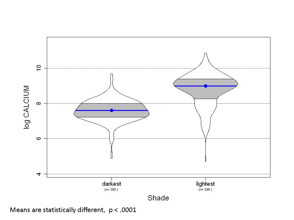
To highlight the differences between the least and the most stable specimens, plot 53 shows the 300 darkest and the 300 lightest specimens pulled from the total of 1,578 specimens analyzed.The vertical axis shows our delta L* scale, which progresses from 0 (white) toward -30 (colors increasingly closer to black). The top and bottom of each ornament represent the highest and lowest values. The gray swelled areas in the middle show the distribution of data between the 25th and the 75th percentiles, and the blue bars with dots in the middle show the means. Plot 54 shows the distribution of both darkest and lightest by year. A reasonable distribution of dates is apparent in both groups. Plots 55 and 56 indicate a statistically significant higher mean for gelatin and calcium in the lighter sheets. Plot 60 shows a statistically significant higher mean for sheet thickness in the lighter sheets as well. On the other hand, plots 57, 58, and 59 show statistically significant higher means in the darker sheets for K, S and Fe, respectively.
Frost grade = A “ornament” plots subset
To prepare another subset of the full data set, we randomly selected 356 books for grading by Gary Frost, University of Iowa conservator. Based on binding, sewing stations, and other evidence, the final Frost totals were 295 grade-A books (likely as original), 28 grade B (possible intervention from washing or resizing), and 33 grade C (intervention likely). Small as the A set is compared to the full database of 1,578 specimens, it provides a more certifiably “as originally made” group of paper specimens with which to test trends observed in the full data set.
The grade-A sheets were divided into two sets: darkest and lightest, again on the delta L* scale, for comparison purposes. Plots 69 and 70 show the differences in overall delta L* values, and again, the distribution by dates. Once again, a statistically significant higher mean for gelatin and calcium is seen in the lighter sheets (plots 71 and 72) and statistically higher means in the darker sheets are evident for K, S and Fe, (plots 73, 74, and 75, respectively). Thickness was essentially the same for both dark and light groups (plot 76).
Materials and workmanship grade “ornament” plots
Additional ornament plots were done to look for any trends indicating differing papermaker raw material use for different qualities of paper in production. There is a slight trend toward more gelatin and calcium in better quality papers seen in plots 46 and 47. (M&W grade 1 = worst quality paper, grade 5 = best quality paper). There is no trend evident with K or S (likely representing alum) application rates in plots 48 and 49. Curiously, in plot 50 there is some evidence that papermakers were less concerned about higher iron accumulation in poorer quality papers than in higher quality papers where the levels are lower. The most likely explanation for this is intentional sourcing of better quality iron-free water in mills that made superior-quality paper.
When specimens were logged into the database for the first time, we took care not to assign lower M&W grades to papers simply because of their darker color. In other words, a darker paper that exhibited superior formation and freedom from knots and debris still received a higher grade. Nevertheless, rougher, poorer quality paper still tends to be darker in color, as seen in plot 52. This correlates with plot 50 for iron content.
In plot 51, thicker paper appears to be associated with poorer quality paper. This is a surprise, as thicker paper tends to consume more pulp and therefore would normally be associated with more expensive paper. Plot 60, where the lightest papers are also the thickest, also seems to contradict plot 51. The only explanation for thinner papers in the higher M&W grades is that extended beating time tends to produce a higher density more compact sheet, while minimized beating times produce a bulkier sheet. Such extended beating times, if used to produce shorter fiber and better formation quality could well be associated with better quality papers because of the added expense. So overall thinner paper in the higher grades is possible. The contradiction between plot 51 and plot 60 however, remains unresolved.
Color
As discussed under PROCEDURES, our color values, determined with our non–CIE L*a*b* standard UV-Vis-NIR instrument, are reported as delta L*, delta a*, and delta b* values, respectively. The CIE standard can be envisioned as a sphere where the L* axis shows the range from white to black. Increasing positive numbers on the a* axis indicate an increase in the color red, and on the b* axis an increase in the color yellow.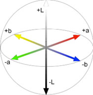
It is common for handlers of historical papers to associate browned paper with brittleness or lack of durability and light-colored sheets with stability or strength. But is there any evidence to support this perception? Our own preliminary analysis of data on thirty-eight historical specimens in a range of conditions from very poor to excellent suggests there is. Data included results from our nondestructive color analyses and small-sample destructive tests for DP (degree of polymerization), pH, ppm calcium, weight percent gelatin, and Pulmac wet zero-span and dry short-span tensile strength (raw and corrected values). Correlations between the variables appear in the matrix below. The boldface red values indeed suggest that darker, redder, or yellower colors can be associated with lower pH, DP, and zero-span (fiber strength) values. This, of course, is in addition to their potentially negative impacts on image or type readability. Experiment B provides details on the analysis methods.
| D L* | D a* | D b* | DP | pH | Gelatin | Calcium | Wet ZS Raw |
Wet ZS Corr. |
Dry SS Raw |
Dry SS Corr. |
|
| D L* | 1 | ||||||||||
| D a* | -0.956 | 1 | |||||||||
| D b* | -0.900 | 0.886 | 1 | ||||||||
| DP | 0.752 | -0.722 | -0.800 | 1 | |||||||
| pH | 0.767 | -0.733 | -0.833 | 0.8919 | 1 | ||||||
| Gelatin | 0.519 | -0.486 | -0.449 | 0.4996 | 0.487 | 1 | |||||
| Calcium | 0.524 | -0.486 | -0.472 | 0.5380 | 0.670 | 0.471 | 1 | ||||
| Wet ZS Raw | 0.755 | -0.706 | -0.739 | 0.8262 | 0.798 | 0.458 | 0.487 | 1 | |||
| Wet ZS Corr. | 0.728 | -0.699 | -0.741 | 0.8535 | 0.820 | 0.423 | 0.447 | 0.908 | 1 | ||
| Dry SS Raw | 0.645 | -0.637 | -0.555 | 0.6579 | 0.575 | 0.494 | 0.338 | 0.835 | 0.707 | 1 | |
| Dry SS Corr. | 0.586 | -0.610 | -0.512 | 0.6575 | 0.568 | 0.466 | 0.268 | 0.693 | 0.774 | 0.870 | 1 |
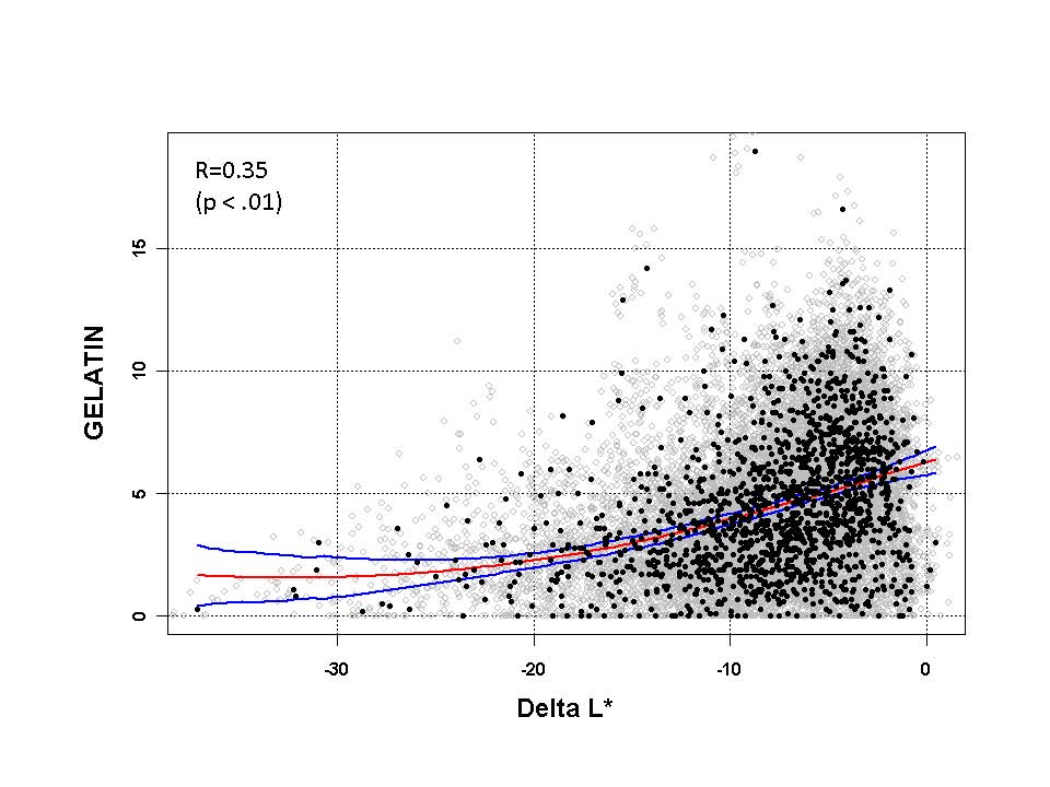
Other trends of interest include plot 17 which shows that delta L* values move toward white (0) as gelatin concentration increases. Plot 18 shows an even stronger trend for Ca. Plots 19 and 20 associate a decrease in K and S levels with whiter color, but the trend is weak. In plot 21, the trend with Fe is more obvious: less Fe results in lighter color.
In plot 23 delta L* versus weight percent alum on calcium carbonate, a large concentration of specimens appears where the lowest percentages of alum are associated with the colors closest to white. As alum percentages increase, relatively fewer specimens are associated with the whitest colors. The same trend is evident in plot 22 Delta L* versus weight percent alum on gelatin.
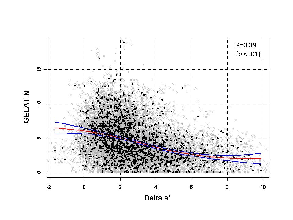
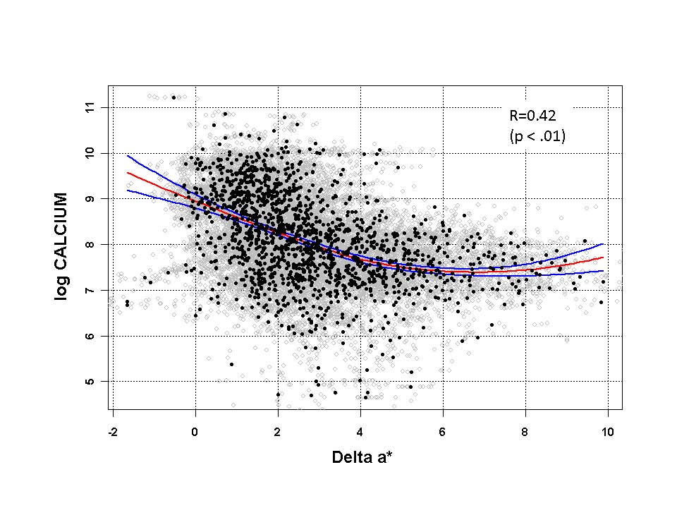
Plot 24 shows that delta a* values trend toward red as gelatin concentration decreases. Plot 25 shows an even stronger trend for Ca: increase in red color as Ca decreases. Plots 26 and 27 show virtually no effect of K and S levels on red color but in plot 21, a slight trend shows increasing Fe associated with increasing red color.
As is the case with delta L*, alum concentration relative to calcium carbonate and gelatin also has a bearing on delta a* values. In plot 30 delta a* versus weight percent alum on calcium carbonate, the lowest percentages of alum are associated, in a large concentration of specimens, with the least red colors. As alum percentages increase, relatively fewer specimens appear associated with the least red colors. The same trend is evident in plot 29 delta a* versus weight percent alum on gelatin.
As a general observation we found little change in delta b* values as the concentration of variables tested changed. Therefore, no delta b* plots are shown.
Interior versus edge
As discussed in PROCEDURES, analyses were done at the edge of each specimen as well as in the interior, primarily to look for evidence of airborne elemental intervention and/or the possibility of significant migration of material toward the edge of the sheet during drying. In Plots 40 and 41, we see little or no indication of this for gelatin or calcium, respectively. Note the gray interior = exterior line in each plot. Equal distribution of symbols on either side of this line suggests no bias in interior versus edge distribution of gelatin or Ca. In plot 42 there is more spread of the symbols but still little evidence of more Fe in the interior of the sheet versus the edge. In plot 43 for S, however, there is a noticeable indication of higher S levels at the edge of the sheet. We interpret this to be evidence of airborne sulfur dioxide or other sulfur-compound deposition at the edge of the sheet. Migration of S-bearing compounds such as alum during drying does not seem likely as there is little evidence of this effect for gelatin, Ca and Fe. Again, no edge data for S was included in any other plots for S or alum. This was the case for all other variables as well: edge data was incorporated only in plots 40, 41, 42, and 43 discussed here.
“Same book, different papers” (SBDP) subset
Many of the trends evident in the nonchronological plots support the trends found in the chronological plots: Ca and gelatin continue to be associated with lighter colored paper, while alum and Fe can be considered to be associated, although in a less robust way, with darker colors. But a problematic and obvious bias remains in the data set: fifteenth-century and earlier artifacts, because of their rarity and place in history, have almost certainly been stored in better conditions over the centuries. Without some way to document storage conditions, any study of papers subjected to long-term natural aging is suspect.
Interestingly, the SBDP subset provides just such documentation. In 229 of the books tested, we found two or more papers in clearly different condition, usually with one noticeably darker than the other. Often, but not always, the mould surface indicated a different maker or mill and/or significant differences in formation quality, knots, clumps, etc.
Sometimes both sheets appeared to be from the same moulds, but their condition was clearly different. Cathleen Baker, in her analysis of nineteenth-century hand and machine papermaking in America, explains this phenomenon by citing discussions in papermaking manuals of “Monday paper” and “Saturday paper.”1 The Monday paper was sized with a fresh batch of gelatin. The Saturday paper was sized in the same solution, which by the end of the week was dirty and/or perhaps loaded up with alum to make the size last through the week without spoiling. It is possible that something similar to this routine was in use throughout the history of the craft.
For this special subset, as for all the other specimens tested, we have no record of storage conditions over time. However, in each SBDP subset book we have two pieces of paper that display very different degrees of stability and they come with the valuable assurance that they have been stored in the same conditions. Even though the specifics of those conditions are unknown, each of these books effectively represents an individual “time capsule” or aging experiment. As such, this subset is perhaps the most important of the entire project. There may be exceptions to this assumption, as when two books are disbound and rebound together again as a single book. But evidence of two or more books bound as one was rare in our specimen set, and to qualify for this subset the two specimens tagged had to be from the same “book.”
The SBDP subset counts by century are as follows:
Century |
Book Count |
Percentage of Total |
1400s |
62 |
27 |
1500s |
55 |
24 |
1600s |
56 |
25 |
1700s |
17 |
7 |
1800s |
39 |
17 |
TOTAL |
229 |
100 |
While we are considering additional ways to utilize the SBDP data, “slope” plots similar to plot 77 give us a good overview of the results. To generate the slope plots, in each century-by-century subplot, any two symbols connected by a line are from the same book. One is darker, and it is paired to a mate that is lighter on the vertical delta L* axis. If the lighter of the two is higher in gelatin content, the line between them has a positive slope and is colored blue. If the darker of the two is actually higher in gelatin content, the slope of the line is negative and the line is colored red. A relatively small difference in gelatin between two papers results a steeper slope and thus a higher number, positive or negative, appropriately weighting the value. A slope caused by a major difference in gelatin content with not much change in delta L* results, appropriately, in a slope closer to horizontal and a number closer to 0. Thus we can see a general effect by net slope for each century. The overall slope effect is reported in the lower right, along with the standard error and a P value indicating statistical significance.
How do the P values indicate statistical significance in the SBDP subset?
Referring again to plot 77, if there were no relationship between delta L* and gelatin over all candidate paper specimens from the fifteenth century, then the chances that we would see a slope coefficient (viz. 0.584) so far from 0 in our small sample is just 0.00078 or .0078%. Because this probability (the P value) is so small, we reject the hypothesis that there is no relationship between delta L* and gelatin. We say that there is statistically significant evidence (P value = 0.00078) of a linear relationship between delta L* and gelatin for fifteenth-century paper specimens. In other words, for the fifteenth-century specimens, for any particular book, a one-unit increase in delta L* is associated with an estimated 0.584-unit increase in gelatin.
As another example, if there were no relationship between delta L* and gelatin in the candidate paper specimens in any of the centuries, then the chances that we would see an overall slope coefficient (viz. 0.786) so far from 0 in our small sample is < 1e-4 (or < 1 in 10,000). We interpret the “overall slope” by assuming that the slopes are the same across the centuries (i.e., assuming the delta L* and gelatin relationship is the same across the centuries), and estimate the common slope within any century as 0.786. Within any century (i.e., controlling for century effects), and for any particular book (i.e., controlling for book effects), a one- unit increase in delta L* is associated with an estimated 0.786-unit increase in gelatin (P value < 1 in 10,000).
Therefore our evaluation of plot 77 is that there is an overall positive effect of gelatin on delta L* values. Inclusion of the nineteenth-century specimens is debatable due to the introduction of chlorine bleaching early in the nineteenth century, which lightened paper color “artificially,” and the decline of gelatin use due to the arrival of rosin and alum internal size at about the same time.
The impact of the different variables on delta L* can be seen in plots 77, 78, 79, 80, and 81. Plots of the impact on delta a* are in development.
Perhaps the best way of assessing the data in the SBDP subset is via the summary of overall slopes and P values in the table below. Note that slopes for a given variable can be compared, century to century, but the overall slopes cannot be compared between variables due to the differences in units and ranges.
SLOPE |
Standard Error |
P value |
||
DELTA L* vs |
Gelatin |
0.786 |
0.102 |
<0.0001 |
Log Ca |
2.884 |
0.271 |
<0.0001 |
|
Log K |
-0.854 |
0.347 |
0.0138 |
|
Log S |
0.248 |
0.27 |
0.358 |
|
Fe |
-0.013 |
.002 |
<0.0001 |
|
Trends in the full data set or in other subsets discussed above are again seen here in the SBDP subset. Gelatin and especially Ca are associated with lighter delta L* color. K is negatively associated with delta L* here, a trend seen earlier in plots 19, 57, and 73. Why the same expected trends with S are not seen in the SBDP subset slope plots is unclear.
Impact trends from the SBDP subset
To further explore this subset, a linear mixed-effects model with a book-specific random intercept was used to evaluate the relative impact of the variables tested on our measures of stability: delta L* and delta a*. Our statistical worksheet provides related details. Note that “impact” in the results below can infer either a positive or a negative influence. Gelatin can have a positive influence, and Fe a negative impact, but they can be ranked first and second in terms of their overall impact on the stability measure. For clarity, variables with a positive influence are shown in boldface. This detail is complicated somewhat by the fact that our delta L* scale runs from 0 to -40 (white to black) and our delta a* scale from 0 to 10 (light to red).
Results are as follows:
Delta L* impact ranking: Ca > Fe > Gel > K
Disclaimer: The impacts of the first four of these covariates look very similar. The S effect is not statistically significant and hence is not included in the impact rankings.
Delta a* impact ranking: Ca > Fe > Gel > K
The S effect is not statistically significant and hence is not included in the impact rankings.
We believe these rankings suggest that Ca and gelatin are relatively strongly associated with lighter color and Fe with redder color in the SBDP subset. This corresponds with the trends seen earlier in plots 17, 18, 21, 24, 25, 55, 56 and 59. Impact rankings and our statistical worksheet for the full data set follow below and confirm the same trends.
Delta L* impact ranking for all 1,578 specimens: Fe > Gel > Ca > K > S
The impacts of the first three covariates are statistically similar.
Delta a* impact ranking for all 1,578 specimens: Gel > Fe > Ca > K > S
The impacts of the first three covariates are virtually identical.
Foxing
In 219 of the 1,578 specimens tested, we subjectively noted the presence of “significant foxing.” The table below shows the average and median observed values for 1,358 specimens without foxing and 219 specimens with foxing. M&W refers to materials and workmanship grade. The differences seen are not considered significant based on our analysis methods. The inability of our analysis criteria to explain the foxing phenomenon suggests that storage conditions—which we were unable to measure—may have played a role. Lower overall Ca and gelatin content could play a secondary role, but more research would be necessary to demonstrate this.
FOXING |
M&W |
S ppm |
K ppm |
Ca ppm |
Fe ppm |
Cl Peak |
Delta L* |
Delta a* |
Gelatin Wt. % |
Ave. w/o Foxing |
3 |
1448 |
737 |
5596 |
389 |
6 |
-7.2 |
2.5 |
4.8 |
Ave. w Foxing |
2 |
960 |
552 |
3157 |
425 |
5 |
-11.5 |
4.3 |
3.1 |
Median w/o Foxing |
3 |
907 |
546 |
3393 |
375 |
5 |
-6.4 |
2.3 |
4.4 |
Median w Foxing |
2 |
632 |
443 |
2393 |
408 |
4 |
-10.9 |
4.2 |
2.6 |
[1] Cathleen A. Baker, From the Hand to the Machine: Nineteenth-Century American Paper and Mediums: Technologies, Materials, and Conservation (Ann Arbor, MI: The Legacy Press, 2010).